To Freeze or Not to Freeze? Training whole-slide models end to end
TMLR · 2026
Summary
Whole-slide pathology models usually keep their image encoder frozen. One big reason is that even small encoders can easily overwhelm GPU memory because histopathology images are too large. In this work, we make the full encoder trainable by processing the input in smaller chunks and moving or recomputing intermediate tensors as needed. This lets a relatively small pathology model (H0-mini) compete with much larger frozen models on an external dataset. On another dataset, freezing still wins. So, when should we let the encoder learn?
One slide, thousands of images, one label
Imagine training an image classifier on a $50,000 \times 50,000$-pixel image. That’s $2.5$ billion pixels. And that’s just one pathology image called a Whole-Slide Image (WSI).
We normally manage this by splitting up the WSI into small images (tiles). An encoder takes each tile and turns it into an embedding (a list of numbers which is a representation of what it sees). A second model (the Multiple Instance Learning (MIL) head) then takes all of those embeddings from all the tiles and makes a prediction about the whole slide (e.g. does it contain a metastasis, what is its prostate cancer grade etc).
We do it because we generally only have a label for the whole slide and not for each individual tile. The model has to work out which bits of the WSI are actually relevant.
There is a catch, though. In the usual pipeline, the encoder is frozen. Its weights stay fixed, and only the MIL head learns.
That encoder could be an ImageNet-pretrained CNN or a massive pathology foundation model. Either way, freezing will lock its features. If the encoder ignores a subtle visual cue your task depends on, too bad—the MIL head has to make do with what it gets.
Why do we accept this? Speed and avoiding overfitting are fair arguments. But let’s be honest about the biggest reason: training the whole pipeline at once simply blows up GPU memory.
How does a small model fill a big GPU?
A ResNet-18 has roughly $11$ million parameters. Its weights take up less than $50$ MB. Surely we can train that on a modern GPU?
For ordinary images, yes. For a WSI represented by hundreds or thousands of tiles, the weights are barely the problem.
As an image passes through the network, each layer computes intermediate values. During training, backpropagation needs some of these values to compute gradients (stuff required to update the model’s weights/parameters). The framework normally keeps those values in VRAM (the GPU’s memory) until the backward pass gets there.
Now do that for every tile, through every layer. Suddenly, a tiny $50$ MB model is demanding hundreds of gigabytes of VRAM just to hold its outputs.
Freezing the encoder completely gets rid of this. With the encoder not going through a backward pass you can extract the tile embeddings with very low memory, write them out to disk and then train the MIL head very cheaply on those pre-computed embeddings.
That convenience, however, leaves an uncomfortable question hanging over the field: are frozen features actually better for generalisation, or are they just the only thing we could fit on our GPUs?
We wanted to make full end-to-end (E2E) training feasible and then test that question.
CNNs: let the GPU work on one piece at a time
If the activation map of a CNN layer is too big for the GPU then we just put it in CPU RAM (a lot cheaper and far more available). The huge tensor stays on the CPU and we feed it to the GPU in chunks. For a memory intensive convolution we just take one chunk over to the GPU, do the normal forward pass, write the output back to RAM and move on to the next chunk.
During backward we bring back the information we need for each chunk and accumulate its gradient contributions. The layer still learns from the full input.
Play animationShow final diagram
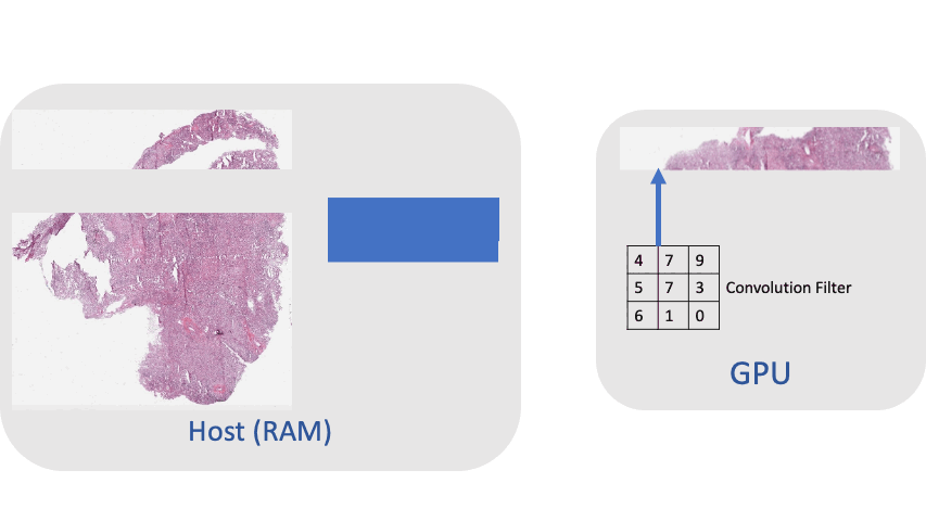
We call these Big Layers: ordinary layers whose computations can handle an input too large to fit entirely on the GPU. Once the activations become small enough, the remaining network can run on the GPU normally. Cheap operations such as ReLU can run on the CPU where that avoids unnecessary transfers.
BatchNorm needs a little more care
A convolution needs nearby pixels. Batch Normalisation needs statistics over the complete tensor used by the layer.
Normalising each chunk separately would give us different statistics and hence change what the network computes. So we use two passes:
- Visit all chunks to accumulate the global mean and variance.
- Visit them again and normalise each chunk using those same global statistics.
Backward also accumulates the global quantities it needs before computing the local gradients. This lets us keep BatchNorm’s behaviour rather than remove it to make the memory problem easier.
That is what we mean by full E2E training here: the slide-level loss updates the MIL head and every trainable encoder layer, using every tile in the selected training bag. It doesn’t mean that every training step uses every available tile from the original slide. We still sample training bags, as MIL pipelines commonly do.
ViTs: keep the embeddings, recreate the rest
For the Vision Transformer (ViT) encoders in our experiments, we can make the unit of work much larger: treat the whole encoder as one Big Layer.
Here’s why. The encoder processes each WSI tile independently. Self-attention still mixes the tokens within a tile, but different WSI tiles only meet later, inside the MIL head.
So we split the bag into micro-batches, small groups of tiles, and use three phases:
- Encode the tiles. Run each micro-batch through the encoder and keep the final embeddings. Throw away the encoder’s internal activations.
- Train the MIL head on the full bag. Combine all the embeddings, compute the slide-level loss, and backpropagate through the head. This tells us how each tile embedding should change.
- Replay the encoder. Run each micro-batch through it again, this time retaining the activations that are required for the backward pass. Use that micro-batch’s embedding gradients and accumulate its contribution to the encoder update.
Play animationShow final diagram
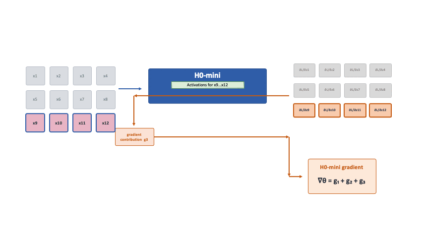
This is essentially whole-encoder gradient checkpointing. We’re spending extra computation to recompute the activations rather than storing and transferring all of them.
Notice what we aren’t doing here: we aren’t taking a shortcut by backpropagating through only a handful of “high-attention” tiles. Every single tile in the bag contributes to the encoder update. Up to standard floating-point quirks, the final gradient is identical to training the whole bag at once.
The MIL head and the final tile embeddings still have to fit on the GPU. They usually need far less memory than the encoder’s intermediate activations, though very large bags can still be demanding, especially for methods that use transformer blocks or other memory-intensive architectures.
Why not use this clean replay trick for CNNs too? Because of BatchNorm. When a layer couples tiles together through shared batch statistics, tiles aren’t independent anymore—which is why CNNs needed our layer-by-layer offloading path instead.
Fine-tuning can also make a model forget
Squeezing the encoder onto the GPU fixes the hardware issue, but that immediately exposes a modelling issue.
Pathology foundation models spend thousands of GPU hours learning rich representations from huge tissue cohorts. If you aggressively fine-tune them on a few hundred slides from one hospital they can overfit to the local idiosyncrasies and lose some of that broad knowledge - a classic case of catastrophic forgetting.
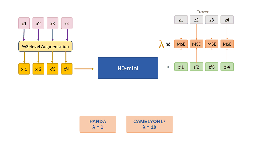
For H0-mini, we use an embedding-matching regulariser inspired by Learning without Forgetting (LwF):
- Before training, we use the frozen pretrained encoder to generate and save reference embeddings for the unaugmented tiles.
- During training, we sample one augmentation setting per slide and apply it consistently to its tiles (WSI-level augmentation).
- Alongside the main slide-classification loss, we penalise the distance between the trainable encoder’s new embeddings and those saved, unaugmented references.
The encoder can adapt to the task, but it also has an incentive to preserve useful aspects of its pretrained representation.
Play animationShow final diagram
So, does letting the encoder learn actually help?
We tested two transfers:
- PANDA to TCGA-PRAD: prostate-cancer grading.
- CAMELYON17 to CAMELYON16: lymph-node metastasis classification.
The first dataset in each pair supplies training data; the second is an external test cohort. We also evaluate on held-out data from the training domain.
We used three MIL heads: ABMIL, DTFD, and TransMIL. For encoders, we studied ResNet-18 (RN18), fine-tuned H0-mini, and several larger frozen pathology foundation models. We tuned the frozen and E2E training regimes separately.
For grading, we report quadratic weighted kappa (QWK), which measures agreement with the reference grades while penalising larger grading mistakes more heavily. As in the paper, we report QWK multiplied by $100$; higher is better. It isn’t classification accuracy.
RN18 needed augmentation to make the external gains convincing
On the in-domain PANDA test set, unfreezing RN18 boosted QWK across all three MIL heads right out of the box. External testing on TCGA-PRAD, however, was much less forgiving.
In fact, naively unfreezing the encoder without augmentation actually made external generalisation worse—dropping ABMIL’s external QWK from $56.34$ to $53.53$. Unfreezing may have given the encoder enough rope to overfit to the source domain.
Once we paired E2E training with WSI-level augmentation, the story flipped completely:
| RN18 setting | ABMIL | DTFD | TransMIL |
|---|---|---|---|
| Frozen + augmentation | 52.83 ± 0.87 | 56.79 ± 4.21 | 36.25 ± 0.78 |
| E2E + augmentation | 65.86 ± 1.73 | 69.47 ± 0.76 | 45.56 ± 7.15 |
The frozen encoder still produces features of augmented images, and the head can learn from them. But only the trainable encoder can change how it represents those variations.
TransMIL’s all-tile result still looks weak here. We’ll come back to that.
A smaller model that can adapt can compete with a larger frozen one
On TCGA-PRAD, H0-mini with E2E + augmentation + LwF could match or exceed the larger frozen encoders we tested. UNI2-h was the strongest larger frozen model in these all-tile comparisons:
| Encoder / training | ABMIL | DTFD | TransMIL |
|---|---|---|---|
| UNI2-h, frozen | 71.10 ± 0.72 | 69.98 ± 0.73 | 55.62 ± 5.98 |
| H0-mini, frozen | 68.63 ± 0.93 | 65.84 ± 2.74 | 54.75 ± 5.84 |
| H0-mini, E2E + Aug. + LwF | 73.38 ± 0.41 | 69.88 ± 0.60 | 70.23 ± 1.82 |
Look at that bottom row: a compact, adapted H0-mini beat frozen UNI2-h with ABMIL ($73.38$ vs $71.10$), crushed it with TransMIL ($70.23$ vs $55.62$), and nearly tied it with DTFD. We also found that, with ABMIL, adapting H0-mini substantially reduced the strong undergrading bias seen on TCGA-PRAD.
Of course, this doesn’t mean small adapted models always beat giant frozen ones—we only fine-tuned H0-mini to stay within a realistic single-GPU budget, not the giant encoders. Still, it shows that task-specific adaptation can punch well above its parameter weight.
CAMELYON gives us the less convenient answer
If this were a typical ML paper, one might have stopped after TCGA-PRAD and declared victory. But our CAMELYON results showed that it isn’t always that simple. On CAMELYON17 (our source domain), the H0-mini adaptation recipe improved test accuracy across all three MIL heads. Great, right? Not so fast. On external CAMELYON16, frozen H0-mini came out ahead. With ABMIL, external accuracy slipped from $97.67\%$ frozen to $96.11\%$ adapted, and DTFD and TransMIL saw similar drops.
The model got better on held-out data from its training hospitals, yet slightly worse on an external cohort. If you only evaluate in-domain, you will fool yourself into thinking fine-tuning is a free lunch. Why the reversal? CAMELYON17 has a much smaller training set than PANDA (442 slides vs 7,647) and an apparently milder domain gap to its external test set—where frozen H0-mini is already near the ceiling at $~97.7\%$.
The training recipe matters, and its ingredients matter differently
The H0-mini results above use a complete recipe. We shouldn’t give all the credit, or blame, to unfreezing.
Our ablations make this clear. For ABMIL on TCGA-PRAD, E2E training alone gave $60.67$ QWK. Adding augmentation brought it to $70.27$, and adding LwF as well gave $73.38$. Across the MIL heads, augmentation accounts for most of the external improvement there; LwF’s extra contribution varies.
On CAMELYON16, the same ABMIL encoder fine-tuned without either component reached only $57.51\%$ accuracy. LwF without augmentation brought it back to $96.63\%$. Here, preserving the pretrained representation made the biggest difference. Even that recovered result remained below the frozen model’s $97.67\%$.
Unfreezing is the starting point. The rest of the training recipe matters a lot!
More tiles at test time can actually hurt
Earlier, we left a cliffhanger: why did TransMIL struggle so badly on TCGA-PRAD when given all foreground tiles?
Look at the bag sizes. During PANDA training, the model sees $256$ tiles per slide (PANDA biopsies are relatively small, averaging $\sim 400$ tiles). External TCGA-PRAD resection slides, on the other hand, average $12,800$ foreground tiles—and go up to $41,000!$
Because TransMIL uses self-attention across tiles, suddenly feeding it $50\times$ more tiles at test time can substantially change the attention patterns it learned during training.
To test that hunch, we capped TCGA-PRAD evaluation at $256$ randomly sampled tiles, matching the training bag size. For E2E RN18 with augmentation, TransMIL jumped from a rough $45.56 \pm 7.15$ QWK (all tiles) to $65.33 \pm 1.14$ ($256$ tiles).
Each trained model was evaluated on $100$ random tile selections and its results were averaged.
ABMIL and DTFD didn’t show the same general improvement from limiting the bag. This supports bag-size shift as part of the explanation for TransMIL’s behaviour. Simply handing an MIL model more tiles isn’t guaranteed to improve its prediction.
What does this cost?
There is no free lunch in systems engineering: we pay for the GPU memory we save with extra compute, CPU RAM, and PCIe data transfers.
The paper includes an FP32 forward/backward benchmark on a 48 GB NVIDIA A40. Native full-bag H0-mini training ran out of memory at both tested bag sizes. With micro-batches of 32, recomputation used approximately:
| Tiles per slide | Native full-bag execution | Micro-batch recomputation |
|---|---|---|
| 256 | Out of memory | 6.78 GiB |
| 512 | Out of memory | 6.79 GiB |
Doubling the bag hardly changed the peak GPU allocation because the encoder still processed only 32 tiles at a time. The extra tiles increased the amount of work.
The wall-clock trade-off is real. On PANDA using a single 24 GB RTX 3090, one epoch takes about $20$ seconds on precomputed features (ignoring extraction time), $45$ minutes when running a frozen RN18 on the fly, $200$ minutes for full E2E RN18, and $255$ minutes for E2E H0-mini. Slow? Yes. Possible on a single consumer-grade GPU instead of crashing immediately? Also yes.
If ordinary E2E training already fits, use it. These methods are useful when that computation would otherwise be impossible within the GPU-memory budget.
So, should we freeze the encoder?
Sometimes! Frozen foundation models remain very strong, and CAMELYON16 gives a clear example of freezing winning.
But on TCGA-PRAD, allowing the encoder to learn from augmentation substantially improved external performance, and adapted H0-mini competed with much larger frozen encoders.
Being able to update the encoder also lets us investigate methods that need to change its representations. For example, the feature-alignment idea in our nuclear-mask paper needs a trainable encoder. We haven’t combined it with this WSI pipeline here, but making that kind of experiment feasible is part of the motivation.
Ultimately, “always freeze” and “always fine-tune” are both wrong. The real question is when adapting the encoder actually helps external generalisation—and now that we can fit the whole pipeline on a single GPU, we no longer have to guess.
You can read the full paper on OpenReview, watch the talk, or look through the code.
For the long road from a course project to this paper, read the story behind Big Layers.
Contributions
- Full end-to-end CNN training within a GPU-memory budget, including BatchNorm with statistics computed over the complete input tensor.
- Micro-batch recomputation for independent ViT tile encoders, retaining the full training-bag gradient.
- Experiments with RN18, H0-mini, three MIL heads, and two source/external dataset pairs, showing when encoder adaptation helps and when it does not.
Citation
Tomar, D., and Kleppe, A. (2026). To Freeze or Not to Freeze? Memory-Constrained End-to-End Training for Whole-Slide Image Classification in Histopathology. Transactions on Machine Learning Research.
@article{tomar2026freeze,
  title   = {To Freeze or Not to Freeze? Memory-Constrained End-to-End Training for Whole-Slide Image Classification in Histopathology},
  author  = {Tomar, Dhananjay and Kleppe, Andreas},
  journal = {Transactions on Machine Learning Research},
  year    = {2026},
  url     = {https://openreview.net/forum?id=ixDBhyLgWs}
}