A Smaller Transformer in Your Transformer
BMVC · 2026

Summary
Vision Transformers seem to spend several consecutive layers doing suspiciously similar work. We replace each group of such redundant layers with one learned Transformer layer. The resulting model has fewer layers and uses much less inference compute while keeping its accuracy close to the original. Sometimes it even beats the larger model on pathology slides!
Wait, what do we mean by “layer” vs. “block”?
Before we get into the fun stuff, let’s clear up some naming chaos.
When a Vision Transformer (ViT) looks at an image, it chops the image up into a grid of small square patches and turns each patch into a list of numbers (its feature representation). From there, the model processes these patches through architecturally identical units called “blocks”. The problem is that when you start studying how groups of these units behave together, you end up talking about “blocks of blocks”. So, we’ll use the following terminology, just like we do in the paper:
-
A layer is a single ViT block.
-
A block is a contiguous sequence of layers stacked one after another (a block of blocks or a group of contiguous blocks).
With that out of the way, let’s talk about why half the layers in your ViT might be slacking off.
Taking four baby steps when one giant leap will do
A typical ViT might have 12, 24, or even more layers. Every time you feed it an image, the patch representations have to go through every single layer sequentially. More layers give the network more capacity to learn complex features during training—but once the model is trained, does it actually need every single one of those steps (layers) at inference time?
Imagine watching someone cross a room by taking four tiny baby steps. If you wanted to copy their journey, you could painstakingly mimic all four baby steps. Or, if you only care about ending up in the exact same spot, you could just take one normal stride and save yourself the effort.
That is the exact premise behind our BMVC 2026 paper, A Smaller Transformer in Your Transformer. We introduce Transformer-Within-Transformer (TWT), a post-hoc method that finds blocks of consecutive layers doing repetitive work in a pre-trained ViT and fuses each block into a single learned layer.
The clue: ViTs take baby steps in phases
How do we know the network is taking baby steps in the first place? Look at what happens to the patch representations as they travel from the first layer to the last. If you measure the cosine similarity between the outputs of every pair of layers, you get a striking pattern: bright yellow squares clustered right along the diagonal.
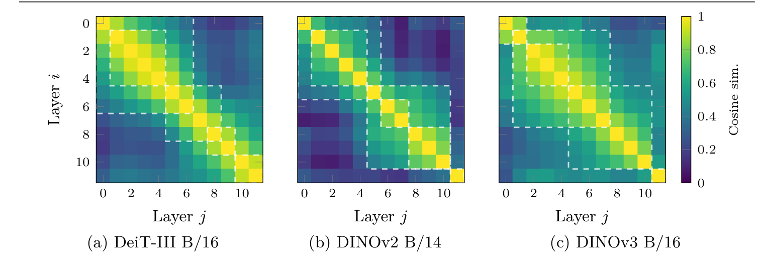
Instead of every layer doing something radically new, the Transformer settles into a handful of distinct computational phases. Inside each phase—empirically a block of contiguous layers—the network is often making tiny, incremental tweaks to the representation. We argue that this step-by-step process isn’t a strict algorithmic necessity; it’s mostly a byproduct of how gradient descent navigates a noisy optimisation landscape during training.
Our starting point was earlier work on this block-diagonal pattern—especially the Block Recurrent Hypothesis (BRH) behind Raptor. But spotting repetitive work is one thing; figuring out what to do with it is where things get interesting. Two existing approaches help set the scene:
-
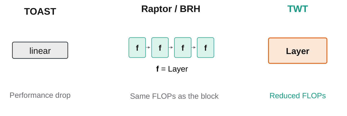
The “Loop It” Approach (Recurrence): Work on the Block Recurrent Hypothesis (like Raptor) argues that since layers in a block do similar things, we can replace a 4-layer block with a single shared layer applied 4 times in a loop. This slashes the parameter count (you only store 1 layer’s weights instead of 4), which is great for memory. The catch? You still have to run that layer 4 times in a row! Your inference compute (FLOPs) stays roughly the same.
-
The “Cheap Shortcut” Approach (Non-Mixing Maps): Methods like TOAST and NOSE go to the opposite extreme. TOAST bridges a redundant block with a simple closed-form linear map, while NOSE removes self-attention from selected layers, leaving their MLPs. This cuts both parameters and FLOPs. The catch? A linear map can’t do dynamic self-attention! Without attention, image patches can’t dynamically mix information, which can lead to a drop in the model’s performance (accuracy).
Our solution with TWT is the best of both worlds. We replace an entire redundant block with one standard ViT layer executed just once. Because it’s a real Transformer layer with self-attention, patches still get to mix information dynamically. And because we run it once instead of looping it $k$ times, we cut inference compute—roughly in half for our six-layer ImageNet models.
How we build a smaller Transformer (in 4 steps)
Turning a 12-layer teacher model into a 4- or 6-layer student model without ruining its brain takes a bit of care. Here is our recipe.
1. Slice the network into blocks (Dynamic Programming)
First, we pass a small calibration set of images through the frozen original model (the teacher) and measure the cosine distance between the intermediate patch representations of possible pairs of layers. For $L$ layers, we get an $L\times L$ matrix.
We want to partition the network’s depth into contiguous blocks where the distance between the start and end of each block stays below a maximum discrepancy threshold $\epsilon$. To find the best split without brute-forcing every combination, we use min-max dynamic programming: we first minimise the total number of blocks $m$ (to get maximum compression). If there’s a tie, we pick the split that minimises the worst-case discrepancy across all blocks. Cranking $\epsilon$ up merges more layers into fewer blocks; dialling it down keeps the model deeper.
2. Hold “auditions” for the replacement layer
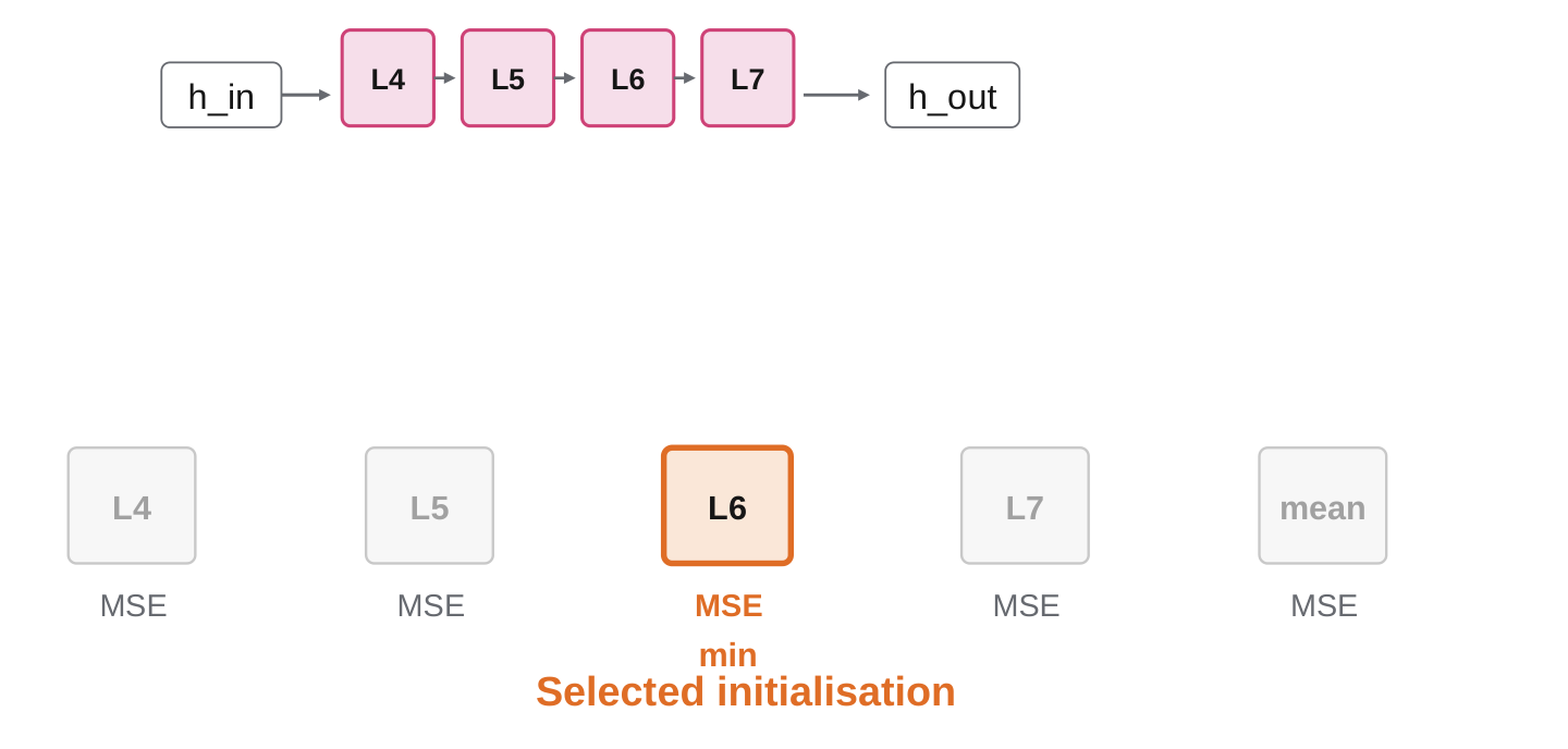
Once we know that, say, Layers 4, 5, 6, and 7 form a single redundant block, we need to initialise the single surrogate layer to replace them. The teacher has already spent all that time learning great features. Why start from scratch?
So, we hold an audition. For a 4-layer block, we line up 5 candidates:
-
Each of the 4 original layers from the block ($L_4, L_5, L_6, L_7$).
-
A 5th “hybrid” candidate created by averaging the weight matrices of all 4 layers (with scaling parameters handled separately).
We train each candidate to mimic the block on a small set of calibration batches. Then we evaluate all candidates on further calibration batches and rank them by the Mean Squared Error (MSE) between the block’s output and the candidate’s output. The candidate with the lowest MSE gets the job as our starting surrogate layer.
Play animationShow final diagram
3. Collapse the blocks
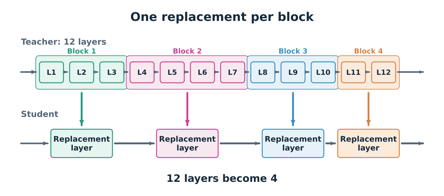
Once every block has an audition winner, we snap them together. If our 12-layer ViT was partitioned into 4 blocks, we now have a 4-layer ViT. Architecturally, it’s 100% a standard ViT—no recurrent loops or special layers required.
Play animationShow final diagram
4. Distil with “check-ins” along the way (Deep Supervision)
Winning an audition gets a layer in the ballpark, but once you stitch 4 surrogate layers together, small approximation errors in Block 1 can snowball by the time you reach Block 4.
After those short auditions, we train our compact student end-to-end in a single global distillation stage using deep supervision. We don’t just tell the student to match the teacher’s final output; we add MSE loss terms at the end of every single block. In plain English, we train the student to reach the same intermediate checkpoints as the teacher, skipping the baby steps in between.
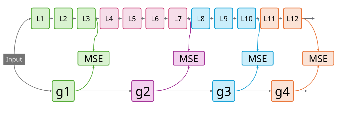
A quick engineering detail on exploding norms: When we looked at natural-image models like DINOv2 and DINOv3, we noticed their representation norms grow exponentially in the deeper layers (DINOv3’s output norm jumps by $63\times$ from the first layer to the last!). When you fuse several layers into one, a single layer struggles to match that massive jump out of the box. For natural images, we add a simple learnable scalar (LayerScale) initialised at 1, and use a staggered cosine schedule that gradually increases the loss weights, with shallower blocks reaching full weight earlier than deeper ones. Once training is done, that scalar is folded right into the layer’s weights—zero overhead!
Interestingly, our histopathology pre-trained models didn’t suffer from exploding late-layer norms at all, so we didn’t even need LayerScale or the staggered schedule for them. Keeping it simple worked right out of the box.
Where compression really shines: Gigapixel Histopathology
A single digitised Whole-Slide Image (WSI) in digital pathology is a gigapixel monster. To analyse one slide, you have to chop it into thousands of tissue tiles, run your ViT backbone on every single tile to extract features, and then feed all those tile features into a Multiple-Instance Learning (MIL) aggregator (like ABMIL or TransMIL) to predict the slide’s cancer grade or metastasis status or whatever else. When you run a backbone thousands of times per slide, saving around 60% or more of your backbone compute per tile adds up fast.
We took two models pre-trained on pathology images—H0-mini and Hibou-B—and compressed them using TWT on prostate biopsy tiles from the PANDA dataset. Then we froze the compressed models, extracted their features, and trained MIL heads on PANDA for prostate cancer grading and CAMELYON17 for detecting breast cancer metastases in lymph nodes. We evaluated them on held-out test splits and completely external cohorts: TCGA-PRAD for prostate grading and CAMELYON16 for metastasis detection.
| Backbone | Method | Layers | FLOPs (G) | TCGA-PRAD (QWK × 100) | CAMELYON16 (accuracy %) |
|---|---|---|---|---|---|
| H0-mini | Baseline | 12 | 23.56 | 69.14 ± 1.22 | 97.31 ± 0.23 |
| H0-mini | TWT | 5 | 9.36 | 70.08 ± 1.08 | 96.73 ± 0.39 |
| Hibou-B | Baseline | 12 | 23.56 | 66.27 ± 1.11 | 90.52 ± 2.48 |
| Hibou-B | TWT | 4 | 7.93 | 67.77 ± 0.67 | 96.16 ± 0.28 |
Here’s the wild part: the compressed TWT models didn’t just match the 12-layer teachers—in several settings, they actually beat them.
Our 5-layer H0-mini cuts parameters from 85.7M down to 36.1M (and FLOPs by ~60%), yet its external prostate grading score on TCGA-PRAD improves by 0.94 points on the QWK × 100 scale with ABMIL (and by a massive 5.87 points with TransMIL!). Similarly, our 4-layer Hibou-B uses just one-third of the original parameters and compute, while jumping from 90.52% to 96.16% accuracy on external CAMELYON16 breast metastasis slides. (It’s not magic across the board, of course—H0-mini dips by about 0.6 percentage points on CAMELYON16, and Hibou-B with TransMIL dips slightly on TCGA-PRAD—but overall, the compressed features generalise shockingly well.)
Putting it to the test: Natural Images (ImageNet-1k)
We also tested TWT on three heavy-hitters in computer vision: DeiT-III, DINOv2, and DINOv3. When we compress these 12-layer models down to 6 layers, we more than halve the parameter count and roughly halve the inference FLOPs, while barely touching top-1 accuracy on ImageNet-1k.
| Backbone | Method | Layers | Params (M) | FLOPs (G) | Top-1 (%) |
|---|---|---|---|---|---|
| DeiT-III B/16 | Baseline | 12 | 86.6 | 17.81 | 83.1 |
| DeiT-III B/16 | TWT | 6 | 39.0 | 8.91 | 82.8 |
| DINOv2 B/14 | Baseline | 12 | 86.6 | 23.42 | 84.6 |
| DINOv2 B/14 | Raptor | 6 RNNs | 39.4 | 23.42 | 84.0 |
| DINOv2 B/14 | TWT | 6 | 39.0 | 11.71 | 84.2 |
| DINOv3 B/16 | Baseline | 12 | 86.6 | 17.82 | 85.2 |
| DINOv3 B/16 | TWT | 6 | 39.0 | 8.92 | 84.4 |
Look at DINOv2 B/14: TWT drops the compute from 23.42 GFLOPs down to 11.71 GFLOPs, and validation accuracy only dips by 0.4 percentage points (from 84.6% to 84.2%)—actually beating Raptor’s 84.0%, even though Raptor still burns the full 23.42 GFLOPs by looping its layers!
Of course, you can’t just keep deleting layers forever. When we pushed compression further to 5 layers, accuracy dropped more noticeably (down to 82.4% on DINOv2). At that point, we’re losing useful information along with the layers.
Same journey, fewer steps?
The point of collapsing a block is to skip its intermediate steps while still reaching roughly the same place. So we wanted to check: does our student still follow the teacher’s broad geometric path through the network?
To look at that, we measured the intrinsic dimension (ID) of the representations across layers using the Two-NN estimator. Think of ID as an estimate of how many independent directions the data vary along: your patch vectors might live in a 768-dimensional space, but the actual surface (or manifold) they trace out might only be 20- or 80-dimensional.
We also applied random colour jitter and spatial augmentations to the input images to see how much the ID estimates wobble at each block boundary.
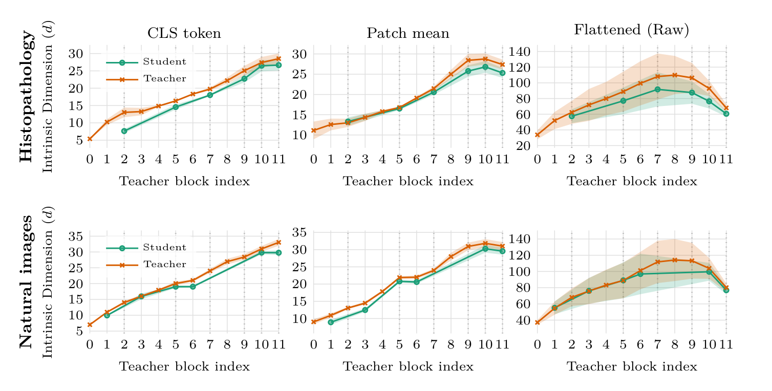
Look at the top-right plot (the raw, unpooled patch representations for histopathology). The green curve (our TWT student) follows the same broad trajectory as the orange curve (the 12-layer teacher), suggesting that our single surrogate layers preserve the broad stages of computation.
But look at the shaded variance bands. For histopathology, the teacher’s ID estimates vary much more across these perturbations—the variance bands are huge! In Table 1’s six-layer H0-mini comparison, the standard deviation of the ID estimates drops by about 38% to 50% at every measured block boundary, and the intrinsic dimension is noticeably lower.
Our hypothesis? Those redundant intermediate baby steps may sometimes accumulate augmentation-sensitive noise instead of useful diagnostic signal. By forcing the network to jump across the phase in a single step, TWT may act as a geometric regulariser, smoothing away some of that variation while keeping the core pathology signal intact. That could help explain why a smaller model sometimes generalises better!
The catch: When do you actually need the baby steps?
We’re big believers in showing where a method breaks, not just where it wins.
Image classification and slide-level MIL are instance-level tasks—you ultimately pool all the patches together to make one decision about the whole image. What happens if we try TWT on a dense prediction task like semantic segmentation (ADE20k), where the model has to label every single pixel?
| Backbone | Method | Layers | FLOPs (G) | mIoU |
|---|---|---|---|---|
| DINOv2 | Baseline | 12 | 147.4 | 47.3 |
| DINOv2 | TWT | 6 | 75.9 | 42.9 |
| DINOv3 | Baseline | 12 | 107.0 | 54.9 |
| DINOv3 | TWT | 6 | 53.6 | 47.4 |
Here, halving the layers hurts noticeably: mIoU drops by 4.4 points on DINOv2 and 7.5 points on DINOv3. Even Raptor (which keeps 100% of the original FLOPs by looping its layers) loses 3.1 and 5.8 mIoU, respectively, though it holds up slightly better than TWT.
Why? Our results suggest that pixel-level segmentation is more sensitive to the fine-grained spatial relationships between patches. While a single attention pass can approximate the macro-step needed for global classification, dense spatial tasks seem to benefit more from gradual, iterative token-mixing across multiple layers. If you’re compressing a model for segmentation, you’ll likely need less aggressive block merging or task-aware distillation.
Wrapping up
The biggest lesson from this project is that architectural depth is not the same thing as algorithmic depth. Just because a Vision Transformer has 12 or 24 layers doesn’t mean it is performing 12 or 24 distinct stages of computation. Often, it’s just taking several baby steps to cross a single computational phase.
By separating the geometry of block redundancy from the surrogate we use to approximate it, TWT gives us a clean, practical way to shrink Vision Transformers after training:
-
Unlike recurrent loops, it actually cuts inference FLOPs.
-
Unlike linear shortcuts, it keeps self-attention intact.
-
And in domain-shifted settings like histopathology, collapsing redundant layers can sometimes boost generalisation on external cohorts—and may be removing some intermediate noise along the way.
If you want to dive into the formulas, explore the ablations on our auditioning step, or see how varying the $\epsilon$ threshold changes the block partitions, check out our full paper on arXiv. And if you want to shrink your own ViTs, the histopathology code for dynamic block discovery, auditioning, distillation, and WSI evaluation is live on GitHub! The conference version is also on OpenReview.
For how the project came together, read the story behind TWT. You can also watch my TWT talk.
Contributions
- A unified geometric view of depth redundancy that decouples layer similarity from how we approximate it.
- Transformer-Within-Transformer (TWT): a post-hoc compression pipeline using dynamic programming for block discovery, candidate auditioning, and single-stage deep supervision.
- Extensive benchmarks across histopathology, ImageNet and ADE20k segmentation—highlighting both where compression shines and where it breaks down.
Citation
Tomar, D., Aasan, M., Kleppe, A., and Ramírez Rivera, A. (2026). A Smaller Transformer in Your Transformer. British Machine Vision Conference (BMVC). Tomar and Aasan contributed equally.
@inproceedings{tomar2026smaller,
  title     = {A Smaller Transformer in Your Transformer},
  author    = {Tomar, Dhananjay and Aasan, Marius and Kleppe, Andreas and Ram{\'{i}}rez Rivera, Ad{\'{i}}n},
  booktitle = {British Machine Vision Conference},
  year      = {2026},
  url       = {https://arxiv.org/abs/2609.20100}
}